
제공된 데이터를 이용해서 부하타입(Load Type) 분류하기
○ 라이브러리 정의
# 데이터 처리
import pandas as pd
# 데이터 분류
from sklearn.model_selection import train_test_split
# HGB , XGB에서 특성중요도 추출라이브러리
from sklearn.inspection import permutation_importance
# 상관관계 검정
from scipy.stats import pearsonr
# 하이퍼파라메터 튜닝
from sklearn.model_selection import GridSearchCV
# 사용할 분류모델들
from sklearn.ensemble import RandomForestClassifier
from sklearn.ensemble import ExtraTreesClassifier
from sklearn.ensemble import GradientBoostingClassifier
from sklearn.ensemble import HistGradientBoostingClassifier
from xgboost import XGBClassifier
# 데이터 스케일링 : 정규화
from sklearn.preprocessing import StandardScaler
# 평가
from sklearn.metrics import accuracy_score
from sklearn.metrics import precision_score
from sklearn.metrics import recall_score
from sklearn.metrics import f1_score
# 오차행렬(혼동행렬)
from sklearn.metrics import confusion_matrix
from sklearn.metrics import ConfusionMatrixDisplay
# 시각화
import matplotlib.pyplot as plt
import seaborn as sns
plt.rc("font",family = "Malgun Gothic")
plt.rcParams["axes.unicode_minus"] = False
# 군집모델
from sklearn.cluster import KMeans
from sklearn.metrics import silhouette_score
# 주성분분석
from sklearn.decomposition import PCA
○ 데이터 불러들이기
import pandas as pd
# 데이터 불러들이기
data = pd.read_csv('data/Steel_industry_data.csv')
data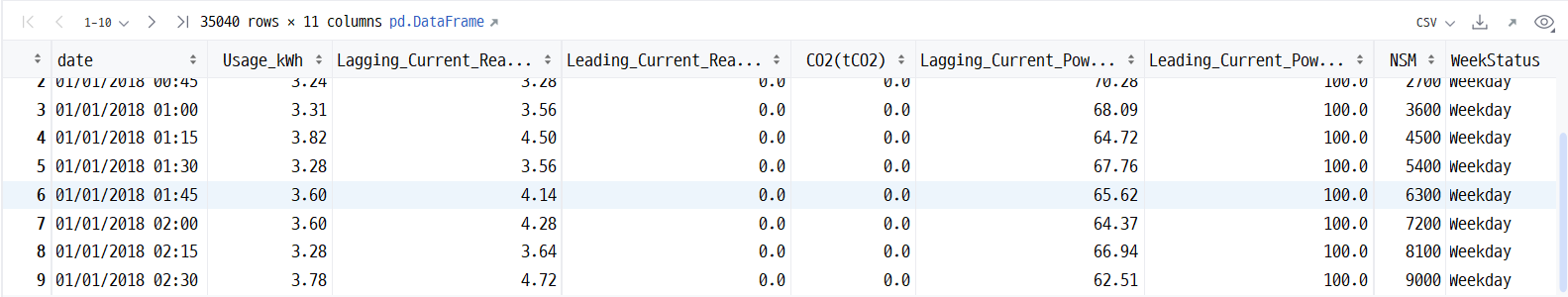
○ 결측치 이상치 확인
# 결측치 확인
data.info()<class 'pandas.core.frame.DataFrame'>
RangeIndex: 35040 entries, 0 to 35039
Data columns (total 11 columns):
# Column Non-Null Count Dtype
--- ------ -------------- -----
0 date 35040 non-null object
1 Usage_kWh 35040 non-null float64
2 Lagging_Current_Reactive.Power_kVarh 35040 non-null float64
3 Leading_Current_Reactive_Power_kVarh 35040 non-null float64
4 CO2(tCO2) 35040 non-null float64
5 Lagging_Current_Power_Factor 35040 non-null float64
6 Leading_Current_Power_Factor 35040 non-null float64
7 NSM 35040 non-null int64
8 WeekStatus 35040 non-null object
9 Day_of_week 35040 non-null object
10 Load_Type 35040 non-null object
dtypes: float64(6), int64(1), object(4)
memory usage: 2.9+ MB
# 이상치 확인
data.describe()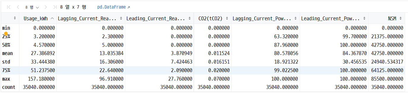
▶ 결측치 이상치 없음
○ 독립변수 종속변수로 분리
# 독립변수 종속변수로 분리
X = data.iloc[:,1:-3]
y = data.iloc[:,-1]
X.shape , y.shape((35040, 7), (35040,))
▶ 총 11개의 컬럼 중 부하타입을 종속변수로 두고 나머지 컬럼들 중에서 날짜와 관련된 컬럼들은 삭제하여
독립변수로 두었다. 날짜 컬럼은 부하타입에 영향을 주지 않기 때문
○ 상관관계
상관관계 확인시 종속변수가 문자열로 되어있으면 확인이 힘들기 때문에 0,1,2의 숫자로 바꿔주는 작업을 진행하였다.
data_temp = pd.concat([X,y],axis=1,ignore_index=False)
for i in range(len(data_temp)):
    if data_temp["Load_Type"][i] == "Light_Load":
        data_temp["Load_Type"][i] = 0
    elif data_temp["Load_Type"][i] == "Medium_Load":
        data_temp["Load_Type"][i] = 1
    else:
        data_temp["Load_Type"][i] = 2
data_temp
숫자로 바꿔준 뒤에 데이터 타입이 문자열로 되어있어 int로 바꿔주는 작업을 하였다.
data_temp["Load_Type"] = data_temp["Load_Type"].astype(int)
data_temp.info()
상관 계수 확인
correlation_matrix = data_temp.corr()
correlation_matrix
상관관계 히트맵 시각화
plt.figure(figsize=(10,8))
plt.title("상관관계 히트맵")
sns.heatmap(correlation_matrix,annot = True , fmt = ".3f" , linewidths = .5 , cmap = "coolwarm")
plt.show()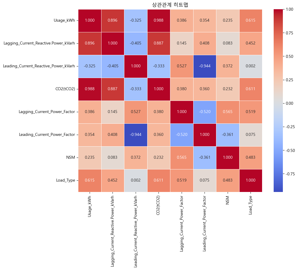
▶해석 :
- 0.01의 값 이하의 상관관계를 가지는 Leading_Current_Reactive_Power_kVarh 의 특성은 Load_Type에 미치는 영향이 적음
- 제거하고 진행하여도 될 정도
- 그러나 제거하지 않고 우선 진행 한 뒤 추후에 제거한 뒤의 성능과 비교해봐야겠다고 판단함
○ 피어슨 상관관계 검정
# 피어슨 상관관계 검정
for column in X.columns:
    corr , p_value = pearsonr(X[column] ,y)
print(f"{column} vs 부하타입 : corr = {corr:.4f} / p-value = {p_value:.4f}")Usage_kWh vs 부하타입 : corr = 0.6146 / p-value = 0.0000
Lagging_Current_Reactive.Power_kVarh vs 부하타입 : corr = 0.4519 / p-value = 0.0000
Leading_Current_Reactive_Power_kVarh vs 부하타입 : corr = 0.0018 / p-value = 0.7395
CO2(tCO2) vs 부하타입 : corr = 0.6107 / p-value = 0.0000
Lagging_Current_Power_Factor vs 부하타입 : corr = 0.5192 / p-value = 0.0000
Leading_Current_Power_Factor vs 부하타입 : corr = 0.0754 / p-value = 0.0000
NSM vs 부하타입 : corr = 0.4828 / p-value = 0.0000
▶ 위 상관관계 히트맵에서와 같이 Leading_Current_Reactive_Power_KVarh 특성의 p-value 가 0.5보다 큰값으로 유의미 하지 않음.
○ 변경된 값으로 독립변수 종속변수 분리
# 독립변수 종속변수로 분리
X = data_temp.iloc[:,:-1]
y = data_temp.iloc[:,-1]
X.shape , y.shape((35040, 7), (35040,))
○ 정규화하기
# 정규화
ss = StandardScaler()
ss.fit(X)
X_scaled = ss.transform(X)
X_scaled
○ 훈련 : 검증 : 테스트 = 6:2:2로 분리하기
# 훈련 : 검증 : 테스트 = 6:2:2 로 분리하기
X_train , X_val , y_train , y_val = train_test_split(X_scaled , y , test_size= 0.4 , random_state=42)
X_val, X_test , y_val, y_test = train_test_split(X_val , y_val , test_size=0.5 , random_state=42)
print(X_train.shape , y_train.shape)
print(X_val.shape , y_val.shape)
print(X_test.shape , y_test.shape)(21024, 7) (21024,)
(7008, 7) (7008,)
(7008, 7) (7008,)
○ 모델 생성하기
# 모델 생성하기
rf_model = RandomForestClassifier()
et_model = ExtraTreesClassifier()
gb_model = GradientBoostingClassifier()
hg_model = HistGradientBoostingClassifier()
xgb_model = XGBClassifier()
모델들을 넣은 리스트 models 만들기
models = [rf_model, et_model , gb_model , hg_model , xgb_model]
models[RandomForestClassifier(),
ExtraTreesClassifier(),
GradientBoostingClassifier(),
HistGradientBoostingClassifier(),
XGBClassifier(base_score=None, booster=None, callbacks=None,
colsample_bylevel=None, colsample_bynode=None,
colsample_bytree=None, device=None, early_stopping_rounds=None,
enable_categorical=False, eval_metric=None, feature_types=None,
gamma=None, grow_policy=None, importance_type=None,
interaction_constraints=None, learning_rate=None, max_bin=None,
max_cat_threshold=None, max_cat_to_onehot=None,
max_delta_step=None, max_depth=None, max_leaves=None,
min_child_weight=None, missing=nan, monotone_constraints=None,
multi_strategy=None, n_estimators=None, n_jobs=None,
num_parallel_tree=None, random_state=None, ...)]
○ 하이퍼파라메터 튜닝
df = pd.DataFrame()
scoring = ["accuracy", "recall" , "precision" , "f1"]
refit = "accuracy"
for model in models:
    modelName = model.__class__.__name__
    gridParams = {}
    print(f"------------[{modelName}]-----------")
    if modelName in ["RandomForestClassifier", "ExtraTreesClassifier","GradientBoostingClassifier"]:
        gridParams["max_depth"] = [3 , 10]
        gridParams["n_estimators"] = [20,40,70]
        gridParams["min_samples_split"] = [2,5,10]
        gridParams["min_samples_leaf"] = [1,5,10]
    elif modelName == "HistGradientBoostingClassifier":
        gridParams["max_depth"] = [3 , 10]
        gridParams["max_iter"] = [50,100,500]
        gridParams["min_samples_leaf"] = [1,5,10]
    else:
        gridParams["max_depth"] = [ 3 , 10]
        gridParams["n_estimators"] = [20,40,70]
        gridParams["min_child_weight"] = [1,5,10]

    print("1------------------------------")
    grid_search_model = GridSearchCV(model , gridParams , scoring = scoring , refit = refit , cv = 5 , n_jobs = -1)
    print("2------------------------------")
    grid_search_model.fit(X_train, y_train)
    print("3------------------------------")

    best_model = grid_search_model.best_estimator_
    train_pred = best_model.predict(X_train)
    val_pred = best_model.predict(X_val)
    test_pred = best_model.predict(X_test)
    train_acc = accuracy_score(y_train , train_pred)
    val_acc = accuracy_score(y_val , val_pred)
    test_acc = accuracy_score(y_test , test_pred)
    pre = precision_score(y_test, test_pred,average="micro")
    rc = recall_score(y_test , test_pred,average="micro")
    f1 = f1_score(y_test,test_pred,average="micro")
    cm = confusion_matrix(y_val, val_pred)


    print(f"1. 최적의 파라메터들(best_params_) : {grid_search_model.best_params_}")
    print(f"2. 성능평가결과[정확도](best_score_) : {grid_search_model.best_score_}")
    print(f"3. 최적의 모델(best_estimator) : {grid_search_model.best_estimator_}")

    df_temp = pd.DataFrame([[modelName, train_acc,val_acc ,test_acc,pre,rc,f1 ]], columns=["모델이름", "훈련정확도","검증정확도","테스트정확도","정밀도","재현율","f1-score" ])
    df = pd.concat([df , df_temp], ignore_index=True)


print()------------[RandomForestClassifier]-----------
1------------------------------
2------------------------------
C:\Users\user\anaconda3\envs\teamproject3\lib\site-packages\sklearn\model_selection\_search.py:979: UserWarning: One or more of the test scores are non-finite: [nan nan nan nan nan nan nan nan nan nan nan nan nan nan nan nan nan nan
nan nan nan nan nan nan nan nan nan nan nan nan nan nan nan nan nan nan
nan nan nan nan nan nan nan nan nan nan nan nan nan nan nan nan nan nan]
warnings.warn(
3------------------------------
1. 최적의 파라메터들(best_params_) : {'max_depth': 10, 'min_samples_leaf': 1, 'min_samples_split': 2, 'n_estimators': 40}
2. 성능평가결과[정확도](best_score_) : 0.8859872767117214
3. 최적의 모델(best_estimator) : RandomForestClassifier(max_depth=10, n_estimators=40)
------------[ExtraTreesClassifier]-----------
1------------------------------
2------------------------------
C:\Users\user\anaconda3\envs\teamproject3\lib\site-packages\sklearn\model_selection\_search.py:979: UserWarning: One or more of the test scores are non-finite: [nan nan nan nan nan nan nan nan nan nan nan nan nan nan nan nan nan nan
nan nan nan nan nan nan nan nan nan nan nan nan nan nan nan nan nan nan
nan nan nan nan nan nan nan nan nan nan nan nan nan nan nan nan nan nan]
warnings.warn(
3------------------------------
1. 최적의 파라메터들(best_params_) : {'max_depth': 10, 'min_samples_leaf': 1, 'min_samples_split': 2, 'n_estimators': 70}
2. 성능평가결과[정확도](best_score_) : 0.8346647946409682
3. 최적의 모델(best_estimator) : ExtraTreesClassifier(max_depth=10, n_estimators=70)
------------[GradientBoostingClassifier]-----------
1------------------------------
2------------------------------
C:\Users\user\anaconda3\envs\teamproject3\lib\site-packages\sklearn\model_selection\_search.py:979: UserWarning: One or more of the test scores are non-finite: [nan nan nan nan nan nan nan nan nan nan nan nan nan nan nan nan nan nan
nan nan nan nan nan nan nan nan nan nan nan nan nan nan nan nan nan nan
nan nan nan nan nan nan nan nan nan nan nan nan nan nan nan nan nan nan]
warnings.warn(
3------------------------------
1. 최적의 파라메터들(best_params_) : {'max_depth': 10, 'min_samples_leaf': 10, 'min_samples_split': 5, 'n_estimators': 40}
2. 성능평가결과[정확도](best_score_) : 0.8963085719845546
3. 최적의 모델(best_estimator) : GradientBoostingClassifier(max_depth=10, min_samples_leaf=10,
min_samples_split=5, n_estimators=40)
------------[HistGradientBoostingClassifier]-----------
1------------------------------
2------------------------------
C:\Users\user\anaconda3\envs\teamproject3\lib\site-packages\sklearn\model_selection\_search.py:979: UserWarning: One or more of the test scores are non-finite: [nan nan nan nan nan nan nan nan nan nan nan nan nan nan nan nan nan nan]
warnings.warn(
3------------------------------
1. 최적의 파라메터들(best_params_) : {'max_depth': 10, 'max_iter': 50, 'min_samples_leaf': 10}
2. 성능평가결과[정확도](best_score_) : 0.89559519216736
3. 최적의 모델(best_estimator) : HistGradientBoostingClassifier(max_depth=10, max_iter=50, min_samples_leaf=10)
------------[XGBClassifier]-----------
1------------------------------
2------------------------------
C:\Users\user\anaconda3\envs\teamproject3\lib\site-packages\sklearn\model_selection\_search.py:979: UserWarning: One or more of the test scores are non-finite: [nan nan nan nan nan nan nan nan nan nan nan nan nan nan nan nan nan nan]
warnings.warn(
3------------------------------
1. 최적의 파라메터들(best_params_) : {'max_depth': 10, 'min_child_weight': 5, 'n_estimators': 20}
2. 성능평가결과[정확도](best_score_) : 0.8959757707681151
3. 최적의 모델(best_estimator) : XGBClassifier(base_score=None, booster=None, callbacks=None,
colsample_bylevel=None, colsample_bynode=None,
colsample_bytree=None, device=None, early_stopping_rounds=None,
enable_categorical=False, eval_metric=None, feature_types=None,
gamma=None, grow_policy=None, importance_type=None,
interaction_constraints=None, learning_rate=None, max_bin=None,
max_cat_threshold=None, max_cat_to_onehot=None,
max_delta_step=None, max_depth=10, max_leaves=None,
min_child_weight=5, missing=nan, monotone_constraints=None,
multi_strategy=None, n_estimators=20, n_jobs=None,
num_parallel_tree=None, objective='multi:softprob', ...)
▶ grid_search 모델을 훈련시키는 과정에서 오류가 발생함. 그러나 최적의 모델 조건은 출력됨.
종속변수의 범주가 3개 이상인 다중분류인 경우 정밀도, 재현율, f1-score 함수 내에
average = "micro"를 추가해줘야함
각 모델의 정확도, 정밀도, 재현율, f1-score 를 담은 데이터 프레임
df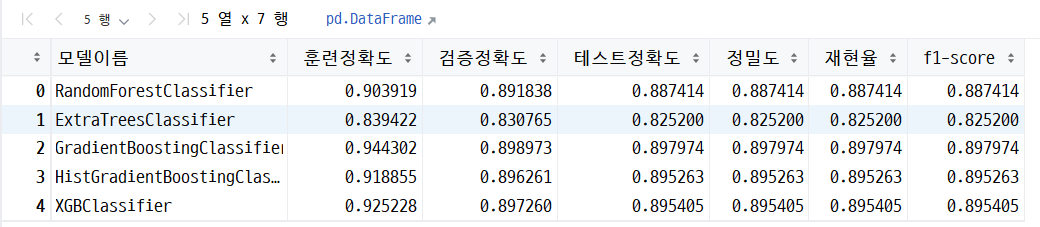
▶ 해석
정확도 : gb > xgb > hgb > rf > et
과적합 여부 : 과소 적합은 일어나지 않음
: 과대적합 (훈련 - 검증 정확도) 의 값이 가장 작은 것은 et , gb 의 경우에는 그 차이가 0.05 정도로 크게 나타남 과대적합(0.1이상차이) 의심됨
재현율 : 재현율이 가장 높은 것은 gb > xgb > hgb > rf > et의 순서
f1-score: 높은것부터 순서는 gb > xgb > hgb > rf > et
최종 선정 모델 : gb
○ 최종 선정 모델로 예측하기
최종 선정 모델 생성
gb = GradientBoostingClassifier(max_depth=10, min_samples_leaf=10,
                           min_samples_split=5, n_estimators=40)
gb
훈련 및 예측
gb.fit(X_train,y_train)
y_pred = gb.predict(X_test)
y_pred
기존 종속변수와 예측 결과 데이터프레임에 저장
data = {
    "test" : y_test,
    "pred" : y_pred
}
test_data = pd.DataFrame(data=data)
test_data
정확도 확인
acc = accuracy_score(y_test , y_pred)
acc0.8972602739726028
○ 군집모델로 분류하기
군집 모델 생성 및 훈련
kmeans_model = KMeans(n_clusters=3 , n_init=10 ,random_state=42)
kmeans_labels = kmeans_model.fit_predict(X)
주성분분석
pca = PCA(n_components=2)
pca.fit(X)
X_pca = pca.transform(X)
군집화 결과 시각화
plt.title("k평균 군집화 결과")
plt.scatter(X_pca[:,0] , X_pca[:,1], c = kmeans_labels)
plt.show()
'머신러닝&딥러닝' 카테고리의 다른 글
| [딥러닝] 신경망 계층 추가방법 및 성능 향상 방법(1) (2) | 2024.01.03 |
|---|---|
| [딥러닝] 텐서플로우 설치 및 중요 개념 정리 (2) | 2023.12.29 |
| [머신러닝] 모델 저장 및 불러오기 (0) | 2023.12.29 |
| [머신러닝] 군집 분류 분석 (1) | 2023.12.28 |
| [머신러닝] 분류 앙상블 모델 (0) | 2023.12.27 |